Overview

This is a guide for mtDNA sequencing data cleaning and analysis in Plink and R.

Learning Objectives

(1) Alignment and variants calling (from fastQ to bam files)

(2) Apply quality control measures for mtDNA genotyping data sets;

(3) Identification of homoplasmic and heteroplasmic variants;

(4) Functional analysis;

(5) Get familiarized with Plink environment.

## All materials are located in the following links: haplocheck_results, haplogroups_workshopsamples.txt, HG0096c_test.bam, HG0097c_test.bam, HG0099c_test.bam, HG0100c_test.bam, HG0101c_test.bam, HG0102c_test.bam, HG0103c_test.bam, HG0105c_test.bam, HG0106c_test.bam, HG0107c_test.bam, Merged.txt, Merged.vcf.gz.

## ***Powerpoint slides for this workshop: Workshop_mtDNA_QC_analysis.pptx

Please download all files and create a folder on your PC or cluster to run the analysis. Remember: plink must be stored in the same folder if running on your PC.

Resources

1. Reference files: Human genome 
   1. Download the reference files using this link https://console.cloud.google.com/storage/browser/genomics-public-data/references/hg38/v0;tab=objects?pageState=(%22StorageObjectListTable%22:(%22f%22:%22%255B%255D%22))&prefix=&forceOnObjectsSortingFiltering=false
2.  Nextflow (https://www.nextflow.io/)
   1. Need to install nextflow in your work directory by using the command: curl -s https://get.nextflow.io | bash
3. Singularity
   1. Need to load singularity module if using CAMH Specialized Computing Cluster: e.g., module load tools/Singularity/3.8.5
4. Mutserve (https://github.com/seppinho/mutserve) 
   1. Need to install mutserve in your work directory by using the command: curl -sL mutserve.vercel.app | bash
5. Our pipeline was adapted from https://github.com/gatk-workflows/gatk4-mitochondria-pipeline.
6. PLINK (http://pngu.mgh.harvard.edu/~purcell/plink/)
   1. PLINK 1.9 (https://www.cog-genomics.org/plink/)
   2. Need to load plink module if using CAMH Specialized Computing Cluster: e.g., module load bio/PLINK/1.9b_6.15-x86_64
7. R (http://cran.r-project.org/)
   1. Need to load R module if using CAMH Specialized Computing Cluster: e.g., module load lang/R/4.0.3-Python-3.8.5-Anaconda3-2020.11
8. Unix-based command terminal
9. A text editor

Before starting

• Download reference files.
• Module load Java, Singularity, and install nextflow and mutserve. 
• Clone your pipeline into your work directory: e.g. git clone pipeline_link_depository

NOTE #1: all written in red is editable.

1. Aligment and variants calling

• To run the alignment and variants calling use the command line below.

#NOTE: Ensure that at the end of the job were created 4 different files for each sample (.vcf, .vcf.tbi, .bam, .bai) and all_samples.csv, and if they were stored inside the folder called output.

Merging the vcf files and obtaining an unique txt files containing all the variants for all the individuals

• For each one of the samples we need to generate an unique .vcf and .txt file that are going to be used for quality control analysis. For that, use the command below.

#NOTE: It is expected to generate two files: Merged.txt and Merged.vcf.gz in the work directory.

#NOTE: all written in red is editable.

Alternative way to merge the vcf files

• If the previous command doesn't work you can use this alternative way to merge all the .vcf files. 

module load bio/BCFtools/1.11-GCC-10.2.0
for i in $(ls *.vcf.gz); do bcftools index --tbi $i; done
bcftools merge -Oz /work_directory/*.vcf.gz -o Merged.vcf.gz

2. Haplocheck

Contamination

wget https://github.com/genepi/haplocheck/releases/download/v1.3.3/haplocheck.zip
unzip haplocheck.zip
./haplocheck --out haplocheck_results Merged.vcf.gz 

3. Haplogrep

Haplogroup

curl -sL haplogrep.now.sh | bash
./haplogrep classify --in Merged.vcf.gz --format vcf --out haplogroups_workshopsamples.txt

• Before go to the Quality Control steps, please download the all_samples.csv and filename.txt files to your computer.

4. Quality Control analysis 

The following files are going to be used for QC analysis: Merged.txt (raw variants data), haplocheck_results (contains the contamination status), and haplogroups_workshopsamples.txt (contains the haplogroup information for each one of the samples).

Filtering out variants from samples identified as contaminated

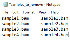
1.  First, to identify the samples that are contaminated we will be using the haplocheck_results file. For that, check the column B (Contaminated Status) and verify if there is any sample indicating YES. If , you will need to copy the Sample IDs (column A: Sample) and paste in a new excel file. Name your file as samples_to_remove and save it as txt format (see the Figure 1 below as an example). 

Figure 1 - samples_to_remove.txt file example.

#NOTE: The samples_to_remove.txt file should have two columns and no header. Both columns have the same information (Sample IDs). This file is going to be used in further steps. If you want, you can already upload this file into your work directory in the SCC cluster.

Quality Control Steps

1. Continue the next steps using the Merged.txt file.
2. First, call the first excel tab as Merged_raw_data.
3. Second, create a 2^nd tab and call it as Merged_nocont. Copy the entire data from the raw results (1^st tab - Merged_raw_data) and paste it into the 2^nd tab. Using the Sample IDs from the samples_to_remove.txt file you will identify the variants from the each one of the contaminated samples and manually remove their respective rows on the Merged_nocont tab.
4. Create a 3^rd tab and call it as coverage>200_both_strand. Copy the entire data from 2^nd sheet (Merge_nocont tab) and paste it into the 3^rd tab. After that, remove all the rows containing variants with coverage lower than 200x in both strands (verify for both CoverageFWD and CoverageREV columns).
5. Create a 4^th tab and call it as Fwd-rev_ratio. Copy the entire data from the 3^rd tab (overage>200_both_strand tab) and paste it into the 4^th. Next, create a new column called FWD-Rev_ratio and calculate the ratio between the CoverageFWD and CoverageREV values (columns L and M). After that, filter out all rows with variants showing Fwd/Rev ratio below 0.5 or higher than 1.5.
6. Create a 5^th tab and call it as remove_del. Copy the entire data from the 4^th tab (Fwd-rev_ratio tab) and paste it into the 5^th . Check the Ref column and exclude all the rows containing the letter N (which means deletion) on this column.
7. Create a 6^th tab and call it as remove_primer_phantom. Copy the entire data from the 5^th tab (remove_del tab) and paste it into the 6^th . After that, remove all the rows containing variants in the primer regions (e.g. 0-500 bp and 16000-16655 bp). Also check if there is any variant at the known phantom mutation sites (72':['G','T'], 257':['A','C'], '414':['G','T'], 3492':['A','C'], 3511':['A','C'], 4774':['T','A'], 5290':['A','T'], '9801':['G','T'], 10306':['A','C'], '10792':['A','C'], '11090':['A','C']). If yes, you should remove the rows containing these variants as well.
8. Create a 7^th tab and call it as homoplasmy_only. Copy the entire data from the 6^th tab (remove_primer_phantom tab) and paste it into the 7^th . Check the VariantLevel column and remove all the rows containing values lower than 95%. 

   #NOTE: Here you can decide for other values such as 97% or 99%, depending on the quality of your sequencing data and the sample size.

9. Create a 8^th sheet in excel and name it as heteroplasmy_only. Copy the entire data from the 6^th tab (remove_primer_phantom tab) and paste it into the 8^th tab. Check the VariantLevel column and remove all the rows containing values lower than 3% and higher than 95%.

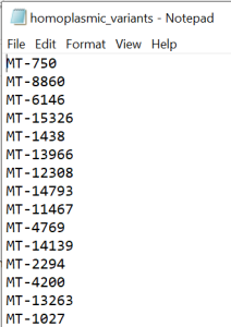
IMPORTANT! After following the QC steps, create a new excel file. Copy and paste the entire data from homoplasmic_only tab into this new excel. Leave only the column containing the variant position (column C: Pos) in the document and exclude the duplicate values. Add MT- ahead to the position of each variant (example MT-73) in Pos column. Remove the header and save as text file called homoplasmic_variants (Figure 2).

Figure 2 - homoplasmic_variants.txt file

#NOTE: The homoplasmic_variants.txt file has only one column with variants names (e.g MT-73) and no header. This file will be further used in the Homoplasmic variants calling step described below and also for statistical analysis.

#NOTE: The homoplasmic_variants.txt file should be uploaded into your folder (directory) in the SCC cluster.

#NOTE: Save the

Homoplasmy and heteroplasmy – transition and transversion rates.

VERY IMPORTANT STEP! It is highly recommended to have at least two people doing together the steps described in this section.

1. Copy the entire data from the homoplasmy_only tab (from Merged.txt file) and paste it into a new excel file. Next, follow the steps described below:

#NOTE: Check out at the end of this section an example of how the excel file was organized in different sheets based on the QC steps (Figure 2).

5. Homoplasmic and common variants filtering using PLINK in the SCC cluster

Converting vcf to plink files

module load bio/PLINK2/20210420-x86_64
plink2 --vcf work_directory_path/Merged.vcf.gz --double-id --max-alleles 2 --vcf-half-call haploid  --make-bed --out Workshop_samples_05-17-23

#NOTE: After running the command above you need to ensure that you got 4 different files called Workshop_samples_05-17-23.bed, Workshop_samples_05-17-23.bim, Workshop_samples_05-17-23.fam and Workshop_samples_05-17-23.log.

• IMPORTANT! Before continuing the analysis, you will need to edit your .bim file by adding the preposition MT- plus the variant location in the second column. For that, you can use the command described below.

awk '{print $1, $1'MT-'$4, $3, $4, $5, $6}' Workshop_samples_05-17-23.bim > Workshop_samples_05-17-23_nv.bim

• After running the command above, I suggest you verify if the new file file_name_outputbim has the MT- added to the variant's position in column 2. For that, you can use the command below.

vi Workshop_samples_05-17-23_nv.bim
ESC :wq

• VERY IMPORTANT! To continue the analysis all the files (.bed, .bim and .fam) need to have the same name. As you changed the .bim file name from Workshop_samples_05-17-23.bim to Workshop_samples_05-17-23_nv.bim remember to change the other files too. For that, you can create a copy of the .bed and .fam files and paste them into a new folder. After doing this, you can manually edit the name of them using the same name structure, such as Workshop_samples_05-17-23_nv.

Filtering out the samples that were contaminated

module load bio/PLINK/1.9b_6.22-x86_64
plink --bfile Workshop_samples_05-17-23_nv --remove samples_to_remove.txt --make-bed --out Workshop_samples_05-17-23_nocont

#NOTE: The samples_to_remove.txt file was created at the QC section.

Homoplasmic variants calling

• For this part of the analysis, you are going to call only the homoplasmic variants by using the txt file. This file was created in the section Quality Control (QC) steps, step 5. Before continuing, you must certify that the homoplasmic_variants.txt file was uploaded into your work directory in the SCC cluster. Next, run the analysis by using the commands described below.

plink --bfile Workshop_samples_05-17-23_nocont --extract homoplasmic_variants.txt --make-bed --out Workshop_samples_05-17-23_nocont_homo

Common variants (MAF ≥ 5%) calling

plink --bfile Workshop_samples_05-17-23_nocont_homo --maf 0.05 --make-bed --out Workshop_samples_05-17-23_nocont_homo_common

6. Functional analysis

./mutserve annotate --input variantsfile.txt --annotation rCRS_annotation_2020-08-20.txt --output AnnotatedVariants.txt

Annotation description

https://github.com/seppinho/mutserve/blob/master/files/rCRS_annotation_descriptions.md

Interpretation of the results

The MutPred score is the probability (expressed as a figure between 0 and 1) that an amino acid substitution is deleterious/disease-associated. A missense mutation with a MutPred score > 0.5 could be considered as 'harmful', while a MutPred score > 0.75 should be considered a high confidence 'harmful' prediction.