Overview
This is a guide for mtDNA sequencing data cleaning and analysis in Plink and R.
Learning Objectives
(1) Alignment and variants calling (from fastQ to bam files)
(2) Apply quality control measures for mtDNA genotyping data sets;
(3) Identification of homoplasmic and heteroplasmic variants;
(4) Functional analysis;
(5) Get familiarized with Plink environment.
## All materials are located in the following links: haplocheck_results, haplogroups_workshopsamples.txt, HG0096c_test.bam, HG0097c_test.bam, HG0099c_test.bam, HG0100c_test.bam, HG0101c_test.bam, HG0102c_test.bam, HG0103c_test.bam, HG0105c_test.bam, HG0106c_test.bam, HG0107c_test.bam, Merged.txt, Merged.vcf.gz, Workshop_samples_05-17-23_nocont_homo_common.bim, AnnotatedVariants.txt.
## ***Powerpoint slides for this workshop: Workshop_mtDNA_QC_analysis.pptx
Please download all files and create a folder on your PC or cluster to run the analysis. Remember: plink must be stored in the same folder if running on your PC.
Resources
- Reference files: Human genome
- Nextflow (https://www.nextflow.io/)
- Need to install nextflow in your work directory by using the command: curl -s https://get.nextflow.io | bash
- Singularity
- Need to load singularity module if using CAMH Specialized Computing Cluster: e.g., module load tools/Singularity/3.8.5
- Mutserve (https://github.com/seppinho/mutserve)
- Need to install mutserve in your work directory by using the command: curl -sL mutserve.vercel.app | bash
- Our pipeline was adapted from https://github.com/gatk-workflows/gatk4-mitochondria-pipeline.
- PLINK (http://pngu.mgh.harvard.edu/~purcell/plink/)
- PLINK 1.9 (https://www.cog-genomics.org/plink/)
- PLINK 2.0 (PLINK 2.0 (cog-genomics.org))
- Need to load plink module if using CAMH Specialized Computing Cluster: e.g., module load bio/PLINK/1.9b_6.15-x86_64
- Unix-based command terminal
- A text editor
Before starting
- Download reference files.
- Module load Java (e.g. module load lang/Java/11.0.6), Singularity, and install nextflow and mutserve.
- Clone your pipeline into your work directory: e.g. git clone pipeline_link_depository
NOTE #1: all written in red is editable.
1. Aligment and variants calling
- To run the alignment and variants calling use the command line below.
| ./nextflow run pipeline_name -r pipeline_version --fastq “/work_directory_path/*_R{1,2}.fastq” -profile singularity --reference /reference_files_path/HG38/references_hg38_v0_Homo_sapiens_assembly38.fasta |
|---|
#NOTE: Ensure that at the end of the job were created 4 different files for each sample (.vcf, .vcf.tbi, .bam, .bai) and all_samples.csv, and if they were stored inside the folder called output.
Merging the vcf files and obtaining an unique txt files containing all the variants for all the individuals
- For each one of the samples we need to generate an unique .vcf and .txt file that are going to be used for quality control analysis. For that, use the command below.
| ./mutserve call --reference rCRS.fasta --output /work_directory_path/Merged.vcf.gz --threads 4 /work_directory_path/filename.bam |
|---|
#NOTE: It is expected to generate two files: Merged.txt and Merged.vcf.gz in the work directory.
#NOTE: all written in red is editable.
Alternative way to merge the vcf files
- If the previous command doesn't work you can use this alternative way to merge all the .vcf files.
module load bio/BCFtools/1.11-GCC-10.2.0 |
|---|
2. Haplocheck
Haplocheck detects in-sample contamination in mtDNA or WGS sequencing studies by analyzing the mitchondrial content. To run haplocheck, you can either use their cloud web service or install it locally.
|
|---|
3. Haplogrep
The haplogroup classifications in Haplogrep are based on the revised tree by Dür et al, 2021, which is an update of the latest PhyloTree version 17 by van Oven, 2016 based on the work of van Oven & Kayser, 2009.
|
|---|
4. Quality Control analysis
The following files are going to be used for QC analysis: Merged.txt (raw variants data), haplocheck_results (contains the contamination status), and haplogroups_workshopsamples.txt (contains the haplogroup information for each one of the samples).
Filtering out variants from samples identified as contaminated
- First, to identify the samples that are contaminated we will be using the haplocheck_results file. For that, check the column B (Contaminated Status) and verify if there is any sample indicating YES. If , you will need to copy the Sample IDs (column A: Sample) and paste in a new excel file. Name your file as samples_to_remove and save it as txt format (see the Figure 1 below as an example).
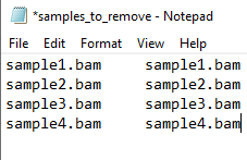
Figure 1 - samples_to_remove.txt file example.
#NOTE: The samples_to_remove.txt file should have two columns and no header. Both columns have the same information (Sample IDs). This file is going to be used in further steps. If you want, you can already upload this file into your work directory in the SCC cluster.
Quality Control Steps
- Continue the next steps using the Merged.txt file.
- Create the first Excel tab named "Merged_raw_data" using the Merged.txt file.
- Create a 2nd tab named "Merged_nocont". Copy the entire data from the raw results (1st tab - Merged_raw_data) and paste it into the 2nd tab. Using the Sample IDs from the samples_to_remove.txt file you will identify the variants from the each one of the contaminated samples and manually remove their respective rows on the Merged_nocont tab.
- Create a 3rd tab named "coverage>200_both_strand". Copy the entire data from 2nd sheet (Merge_nocont tab) and paste it into the 3rd tab. After that, remove all the rows containing variants with coverage lower than 200x in both strands (verify for both CoverageFWD and CoverageREV columns).
- Create a 4th tab named "Fwd-rev_ratio". Copy the entire data from the 3rd tab (overage>200_both_strand tab) and paste it into the 4th. Next, create a new column called FWD-Rev_ratio and calculate the ratio between the CoverageFWD and CoverageREV values (columns L and M). After that, filter out all rows with variants showing Fwd/Rev ratio below 0.5 or higher than 1.5.
- Create a 5th tab and call it as remove_del. Copy the entire data from the 4th tab (Fwd-rev_ratio tab) and paste it into the 5th . Check the Ref column and exclude all the rows containing the letter N (which means deletion) on this column.
- Create a 6th tab named "remove_primer_phantom". Copy the entire data from the 5th tab (remove_del tab) and paste it into the 6th . After that, remove all the rows containing variants in the primer regions (e.g. 0-500 bp and 16000-16655 bp). Also check if there is any variant at the known phantom mutation sites (72':['G','T'], 257':['A','C'], '414':['G','T'], 3492':['A','C'], 3511':['A','C'], 4774':['T','A'], 5290':['A','T'], '9801':['G','T'], 10306':['A','C'], '10792':['A','C'], '11090':['A','C']). If yes, you should remove the rows containing these variants as well.
- Create a 7th tab named "homoplasmy_only". Copy the entire data from the 6th tab (remove_primer_phantom tab) and paste it into the 7th . Check the VariantLevel column and remove all the rows containing values lower than 95%.
#NOTE: You have the flexibility to adjust the threshold values based on the quality of your sequencing data and the specific requirements of your analysis.
- Create a 8th tab named "heteroplasmy_only". Copy the entire data from the 6th tab (remove_primer_phantom tab) and paste it into the 8th tab. Check the VariantLevel column and remove all the rows containing values lower than 3% and higher than 95%.
#NOTE: Check it out an example of how the Merged_QC excel file should be organized in different tabs based on the QC steps described above (Figure 2).
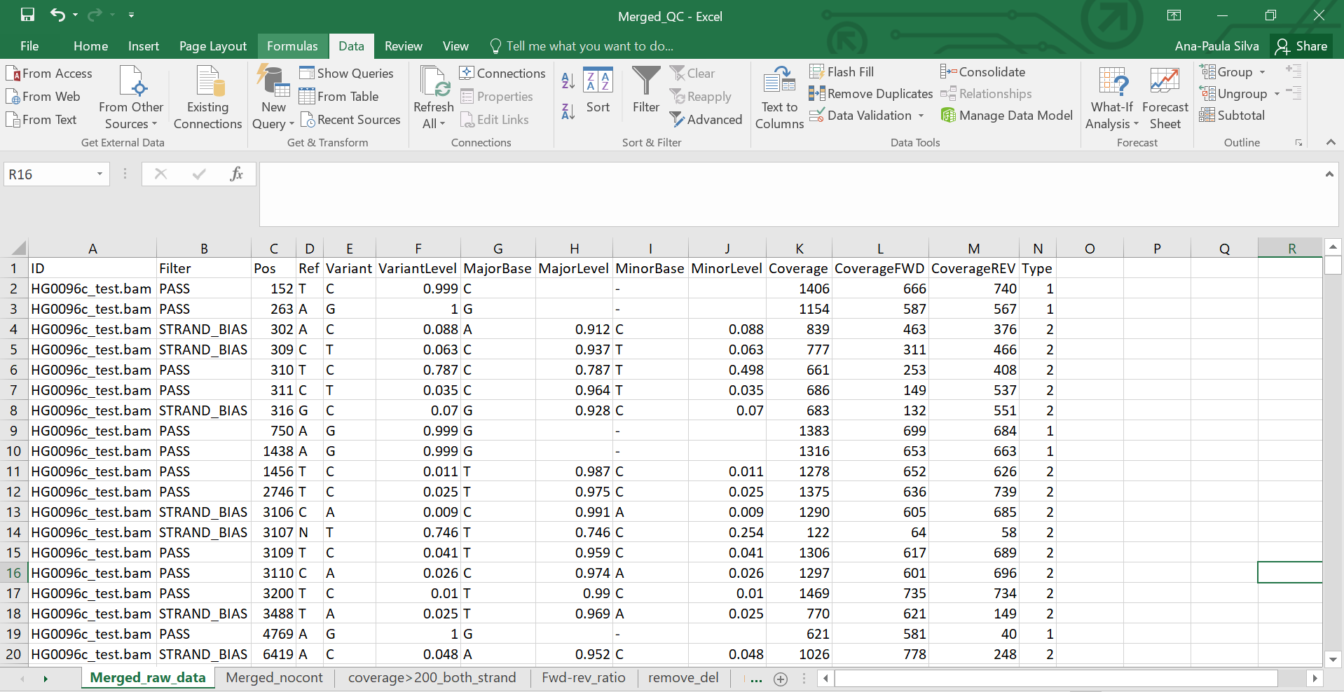
Figure 2 - Merged_QC.csv file example
IMPORTANT! After following the QC steps, create a new excel file. Copy and paste the entire data from homoplasmic_only tab into this new excel. Leave only the column containing the variant position (column C: Pos) in the document and exclude the duplicate values. Add MT- ahead to the position of each variant (example MT-73) in Pos column. Remove the header and save as text file called homoplasmic_variants (Figure 3).
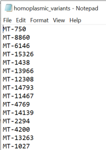
Figure 3 - homoplasmic_variants.txt file
#NOTE: The homoplasmic_variants.txt file has only one column with variants names (e.g MT-73) and no header. This file will be further used in the Homoplasmic variants calling step described below and also for statistical analysis.
#NOTE: The homoplasmic_variants.txt file should be uploaded into your folder (directory) in the SCC cluster.
#NOTE: Save the excel file as Merged_QC.csv.
Homoplasmy – transition and transversion ratio.
VERY IMPORTANT STEP! It is highly recommended to have at least two people doing together the steps described in this section.
- Copy the entire data from the homoplasmy_only tab (from Merged_QC.csv file) and paste it into a new excel file. Next, follow the steps described below.
- First, name the 1st tab as homoplasmic_variants. The first tab contains the total number of variants (number of rows). Take a side note of the total number of variants you have.
- Create a 2nd tab and call it as unique_homoplasmic_variants. Copy and paste the entire data from the 1st tab into the 2nd and exclude all the duplicate variants, this way you are going to keep only unique/bi-allelic variants. Take a side note of the number of unique variants you have at this step.
- Create a new column in the unique_homoplasmic_variants tab called Type_of_mutation. The Type_of_mutation column will show a number that indicates the type of substitution mutation which 1 will refer to a transition type and 2 to a transversion type. In transition, one purine is substituted for another purine or one pyrimidine is substituted for another pyrimidine (Transitions are: A>G, G>A, C>T or T>C). In transversion, a purine base is substituted for a pyrimidine base or vice versa (Transversions are: A>C, C>A, G>T, T>G, G>C or C>G). In figure 4, you can double-check the different types of substitution mutations.

Figure 4 - Type of mutation
- Check out the columns Ref and Variant (columns D and E) and add the value 1 (when you identify a transition) or add the value 2 (when you identify a transversion) type to the column Type_of_mutation.
- Next, take a side note of the total number of transitions and transversions you have into the column Type_of_mutation.
- Calculate the percentage (%) of both transitions and transversions in comparison to the total of unique variants.
- Calculate transition/transversion ratio by dividing the percentage (%) of transitions by the percentage (%) of transversions.
Example:
Total number of homoplasmic variants: 1211
Total number of unique/bi-allelic variants: 335
Number of transitions in comparison to the total number of unique/bi-allelic variants: 325 (97,01%)
Number of transversions in comparison to the total number of unique/bi-allelic variants: 10 (2,99%)
Transitions/transversions ratio Ti/Tv: 32.44:1.
NOTE: The reference ratio of Ti/Tv for homoplasmic variants goes from 20:1 to 38:1.
Heteroplasmy - transition and transversion ratio.
- Copy the entire data from the heteroplasmy _only tab (from Merged_QC.csv file) and paste it into a new excel file. Next, follow all the steps described above for the "Homoplasmy - transition and tranversion ratio" analysis.
#NOTE: There is no established reference ratio of Ti/Tv for heteroplasmic variants.
5. Homoplasmic and common variants filtering using PLINK in the SCC cluster
Converting vcf to plink files
module load bio/PLINK2/20210420-x86_64 |
|---|
#NOTE: After running the command above you need to ensure that you got 4 different files called Workshop_samples_05-17-23.bed, Workshop_samples_05-17-23.bim, Workshop_samples_05-17-23.fam and Workshop_samples_05-17-23.log.
- IMPORTANT! Before continuing the analysis, you will need to edit your .bim file by adding the preposition MT- plus the variant location in the second column. For that, you can use the command described below.
awk '{print $1, $1'MT-'$4, $3, $4, $5, $6}' Workshop_samples_05-17-23.bim > Workshop_samples_05-17-23_nv.bim |
|---|
- After running the command above, I suggest you verify if the new file file_name_outputbim has the MT- added to the variant's position in column 2. For that, you can use the command below.
vi Workshop_samples_05-17-23_nv.bim |
|---|
- VERY IMPORTANT! To continue the analysis all the files (.bed, .bim and .fam) need to have the same name. As you changed the .bim file name from Workshop_samples_05-17-23.bim to Workshop_samples_05-17-23_nv.bim remember to change the other files too. For that, you can create a copy of the .bed and .fam files and paste them into a new folder. After doing this, you can manually edit the name of them using the same name structure, such as Workshop_samples_05-17-23_nv.
Filtering out the samples that were contaminated
- To filter out the contaminated samples we will use the file samples_to_remove.txt created in previous steps on the QC section. Verify if you have already uploaded this file into the work directory and run the commands described below.
module load bio/PLINK/1.9b_6.22-x86_64 |
|---|
#NOTE: The samples_to_remove.txt file was created on the QC section.
Homoplasmic variants calling
- For this part of the analysis, you are going to call only the homoplasmic variants by using the homoplasmic_variants.txt file. This file was created in the section Quality Control (QC) steps. Before continuing, you must certify that the homoplasmic_variants.txt file was uploaded into your work directory in the SCC cluster. Next, run the commands described below.
plink --bfile Workshop_samples_05-17-23_nocont --extract homoplasmic_variants.txt --make-bed --out Workshop_samples_05-17-23_nocont_homo |
|---|
Common variants (MAF ≥ 5%) calling
- Minor allele frequency (MAF) is the frequency at which the second most common allele occurs in a given population. MAF is widely used in population genetics studies because it provides information to differentiate between common, low-frequency and rare variants in the population.
#NOTE: Common (MAF ≥ 5%), low-frequency (0.5 ≤ MAF ≤ 5%) and rare (MAF ˂ 0.5%) variants.
plink --bfile Workshop_samples_05-17-23_nocont_homo --maf 0.05 --make-bed --out Workshop_samples_05-17-23_nocont_homo_common |
|---|
#NOTE: Download the Workshop_samples_05-17-23_nocont_homo_common.bim , open it in excel and save it as common_variants.
Example: Phenotypes and correlation analysis
plink --bfile Workshop_samples_05-17-23_nocont_homo_common --allow-no-sex --linear --pheno phenotype.txt --pheno-name phenotype_interested_measure --out res_phenotype_interested_measure
NOTE: do the command described previously for all phenotype variables you have interest in your data. The type of test used (e.g. linear model, logistic, etc) will depend on the type of data you have.
6. Functional analysis
The effect of mutations-caused amino acid changes on protein function was predicted by a combination of tools that use sequence homology, evolutionary conservation, and protein structural information.
- To run the functional analysis, first you need to create the variantsfile.txt. For that, you will utilize the information from the Workshop_samples_05-17-23_nocont_homo_common.bim file obtained in the previous step. The variantsfile.txt file should be structured with two columns, namely Pos and Variant. For further reference, please consult Figure 5.
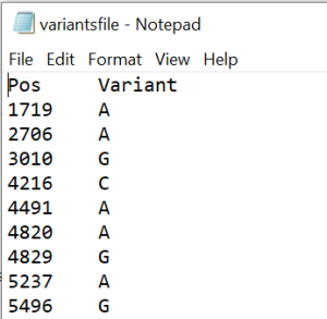
Figure 5 - variantsfile.txt example
2. Upload the variantsfile.txt into your work directory in the SCC cluster and run the command below.
./mutserve annotate --input variantsfile.txt --annotation rCRS_annotation_2020-08-20.txt --output AnnotatedVariants.txt |
|---|
Annotation description
https://github.com/seppinho/mutserve/blob/master/files/rCRS_annotation_descriptions.md
Interpretation of the results
The MutPred score is the probability (expressed as a figure between 0 and 1) that an amino acid substitution is deleterious/disease-associated. A missense mutation with a MutPred score > 0.5 could be considered as 'harmful', while a MutPred score > 0.75 should be considered a high confidence 'harmful' prediction.